
A Practical Guide to Using an Oscilloscope
Learn how to use the oscilloscope, frequently referred to in the trade as a scope, which is an essential diagnostic tool used in any serious electronic circuit design activities.

A scope provides a time-stamped, running clip of a signal at the point of measurement. The signal in this case is simply an input voltage.
The usefulness of a scope lies in knowing what point in the circuit to probe, when to start the actual probing, how to properly set up the scope, and how to interpret what the scope is showing. These are all totally dependent on the skills and knowledge of the scope operator.
Specifically, knowing what kind of signal to expect at a given circuit point, interpreting what is actually happening at that same point, interpreting any deviations, and drawing the appropriate conclusions, is fully up to the operator.
In this article we are going to look at how to properly set up and use an oscilloscope.
How Does an Oscilloscope Work?
With modern scopes, the display is simply a rectangular area with an X-Y grid pattern. This grid pattern can be an actual overlay, or a superimposed image.
The x-axis is time, and it sweeps from left to right. The y-axis displays the sampled voltage value of the input at all points along the time sweep. The display is then just a plot of the input vs time.
It is common to specify the time scale as: ms/div, or us/div, or ns/div, where ms is milliseconds, and us is microseconds and so on, per division. Similarly, the vertical axis is specified as V/div, or mV/div.
To better appreciate this, figure 1 show what the scope displays when the input is a 1KHz sine wave with a peak voltage of 1V. It is easily seen that the amplitude of the signal is 1V, and since the vertical setting of the scope is 1 V/div, the peak of the signal is exactly 1 division high.
Horizontally, there are ten divisions, each with a setting of 100us/div, for a total of 1000us, or 1ms. This is exactly the period of a 1KHz sine wave.
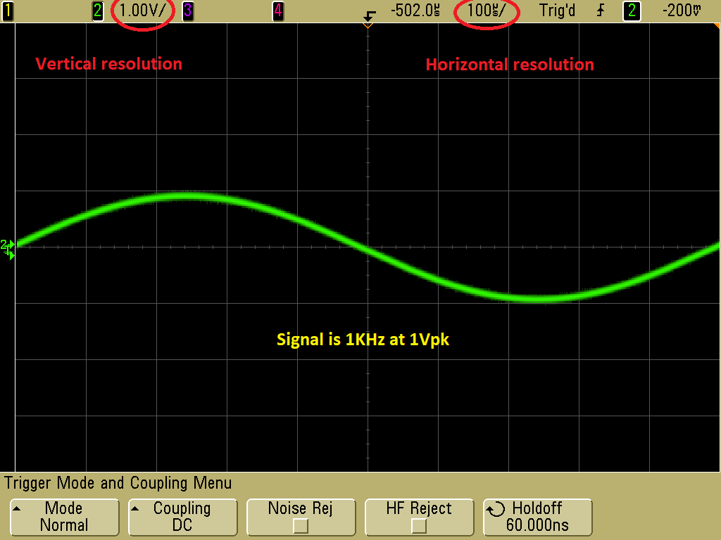 Figure 1 – Scope capture of a 1KHz, 1Vpk sine wave at 1V/div vertical and 100us/div horizontal
Figure 2 shows the same input with the scope horizontal scale set to 200us/div. Now, two complete cycles are displayed.
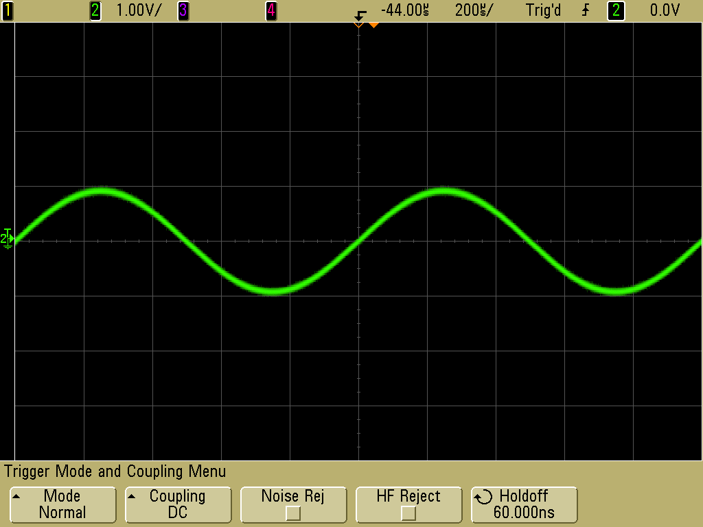 Figure 2 – Scope capture of a 1KHz, 1Vpk sine wave at 1V/div vertical and 200us/div horizontal
Figure 3 is again the same signal but displayed at 500mV/div and 500us/div. From these pictures, it is clear that by manipulating the horizontal and vertical resolutions, more or less of the input signal is displayed.
For example, since the size of the viewing screen has not changed, then viewing just one cycle will show more details, while increasing the time-base of the horizontal shows the larger overall picture, which, in this particular case, is more of the same sinusoidal wave.
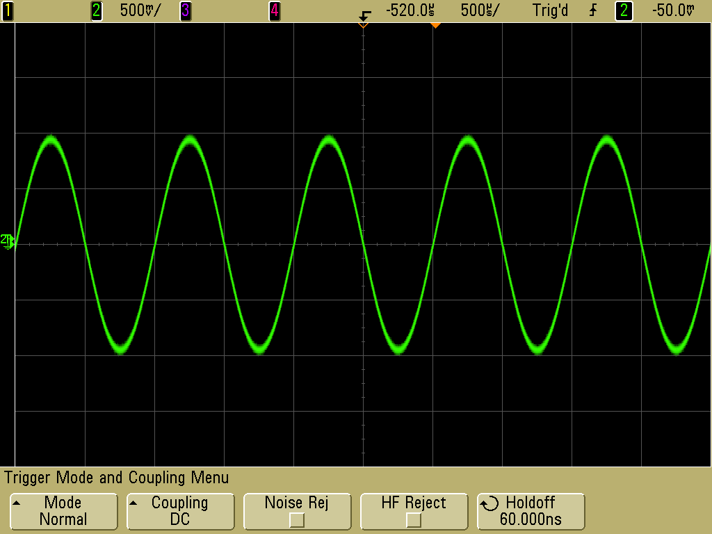 Figure 3 – Scope capture of a 1KHz, 1Vpk sine wave at 500mV/div vertical and 500us/div horizontal
Going back to figure 1, the scope display captured a 1ms clip of the input. That input existed before the capture started, and continued on after that. So, how was the scope able to capture exactly one cycle of this sinusoidal input, starting a 0V?
In other words, since the probing could have started at some random time, how was the scope able to start capturing at the exact time a cycle, one of many, started?
The answer is that all scopes have a trigger level setting. The horizontal sweep starts when the trigger condition is met. In this case, the scope was set to trigger on the input signal itself, with trigger level set to 0V. It was also set to trigger on the rising edge.
These are controls that are available on all scopes, and allow the user to determine exactly when to start the capture, which, again is on the left most part of the display. The trigger could have been set to any value, with rising or falling edge capture.
This trigger signal could also have been selected to be from some other source beside the input signal itself.
This allows the user to precisely determine which section of interest, of the signal, to display.
Figure 4 shows what the display looks like with the trigger level set to 0.5V, rising edge. Figure 6 shows how it looks like with the trigger level set to -0.5V, rising edge.
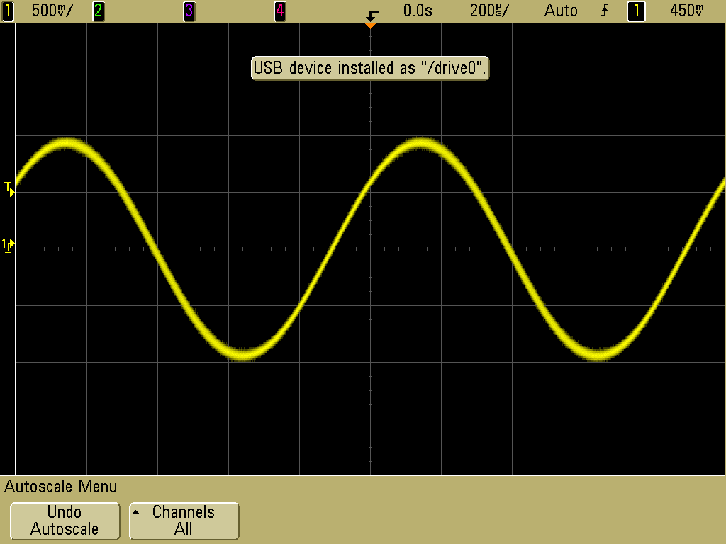 Figure 4 – Scope capture of a 1KHz, 1Vpk sine wave with trigger level set to 500mV, rising edge
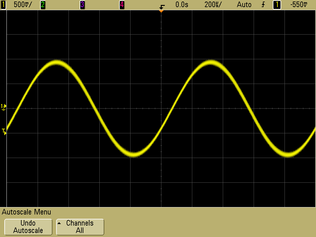
Figure 5 – Scope capture of a 1KHz, 1Vpk sine wave with trigger level set to -500mV, rising edge
Figure 6 illustrates another scenario. It is the 5V DC output of an AC adapter, clearly showing that the adapter’s output in not clean. However, from this capture it is very hard to tell just how much ripple is riding on this 5V line.
You need to remove the 5V DC, and just show the ripple only. This is what figure 7 shows after the coupling mode, another available setting of the scope, has been changed from DC to AC.
You can now clearly see that the ripple is about 200mV.
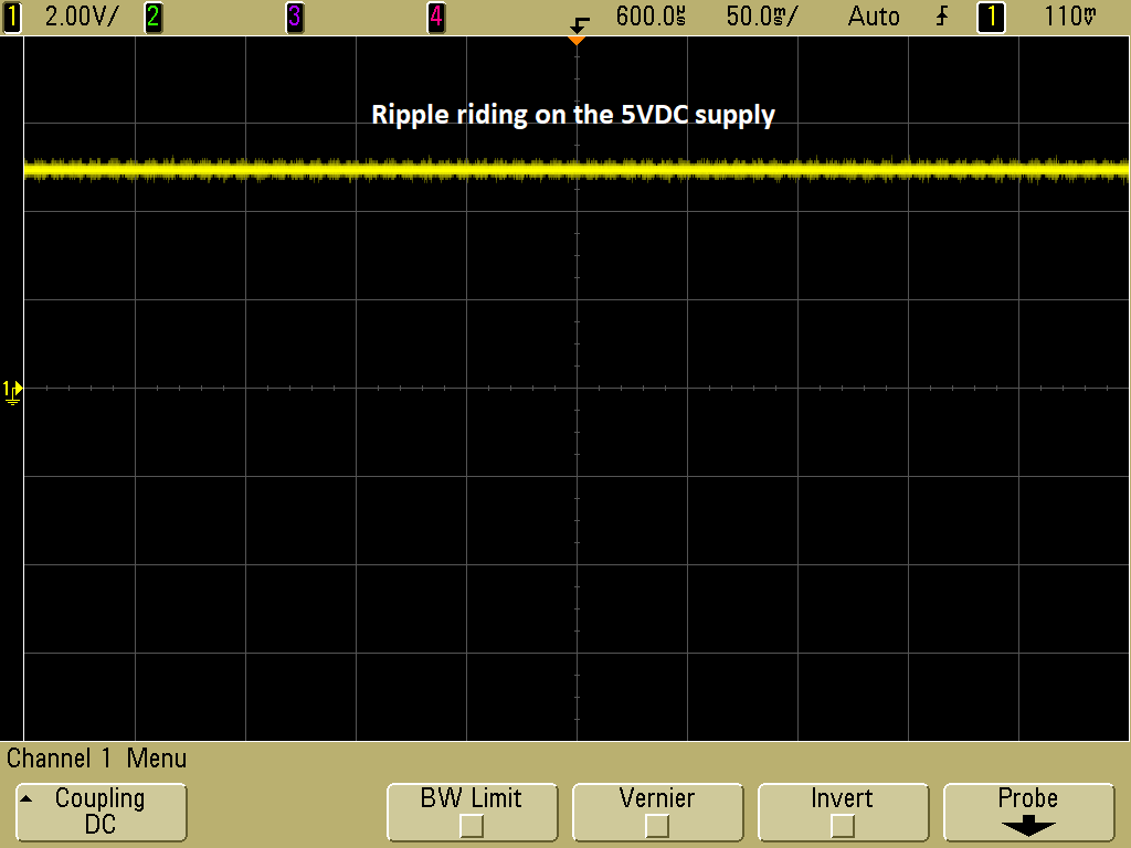
Figure 6 – Ripple on the DC output of an AC Adapter
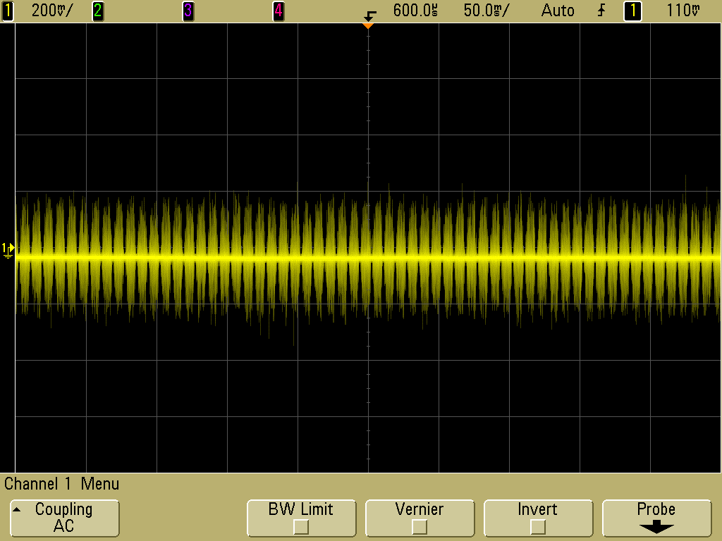
Figure 7 – Actual ripple after removing the DC part through the scope’s AC coupling
Figure 8 shows the main blocks of a basic oscilloscope. It encompasses everything that has been described so far.
There is the time base for the horizontal sweep, with trigger to start it. The trigger source can be derived from the input signal itself, or it can be from other sources.
For the vertical there is a vertical amplifier, with either direct or DC coupling, or through a capacitor for AC coupling.
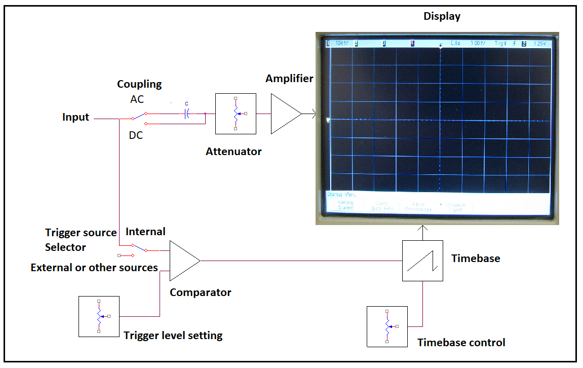
Figure 8 – Main blocks of a simple oscilloscope
Features of Real Oscilloscopes
There are two basic kinds of scopes – analog and digital. The general description presented in the previous section applies to both kinds. However, the older technology analog scopes have been replaced by digital scopes, and the rest of this article will deal mostly with digital scopes.
They have capabilities that are simply not present in analog scopes. For example, analog scopes are mostly real-time instruments. They display the signal as received, and do not have memory or math capabilities. Some specialized analog scopes had screen persistence features, but not anywhere near what digital scopes can do.
While all of the basic features introduced in the previous section are present in all scopes, this section presents even more features, some of which are present in even relatively inexpensive scopes.
The first feature, as mentioned, is memory. All the scope pictures in the previous section were first frozen in the scope’s internal memory, and then saved in a USB flash drive.
Here are some the most common features available in digital scopes:
Multiple channels
Most scopes have at least two input channels, and some have four. A very important feature is to allow viewing multiple signals that have some kind of relationship with each other.
One important thing to note here is that there can only be one trigger source at any one time. However, this trigger source may be on any input channel, or it can be an external trigger that is not based on any of the input signals.
As an example of how this can be used, consider an I2C communication link. Since data is transferred in the falling edge of the SCL line, this edge can be used as the trigger source, and it is then possible to see what the actual data being read is if the SDA line is monitored on the second channel.
A typical example is shown in figure 9. It shows the very first byte of an I2C OLED initialization. Incidentally, since this circuit was actually built on a breadboard for this article, it also shows some cross-talk between the SDA, and SCL lines. However, as seen from the scope capture, it was not enough to affect normal operation.
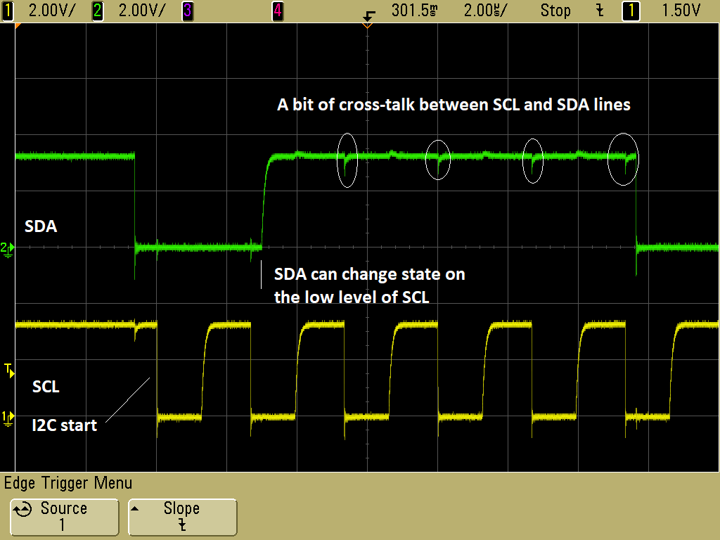
Figure 9 – I2C SCL and SDA captured from an OLED initialization sequence
Pre-trigger and delayed trigger
Since a digital scope is always converting the input signal to digital data, it is also possible to view what happened before the trigger, and to delay the start of the actual signal capture till sometime after the trigger condition.
For example, the trigger condition may be an error flag being asserted, and the pre-trigger feature can show what happened to some other signals just prior to this error flag being asserted. With delayed trigger on the other hand, it is possible to view what happened some pre-determined time after the actual trigger event.
Math functions
Since the data captured is digital, and is in the scope’s internal memory, it is possible to do mathematical computations on the data. A common one is the calculation the RMS and average values of the captured input signal. Some scopes also allow doing FFT and other advanced computations on the input signal.
A very simple, but quite useful, math computation is the displaying of the difference between two input channels of the scope. If the two inputs are actual inputs to a differential amplifier, this function can show what the output of the amplifier should look like.
Another use of that is to actually show the real-time current waveform in a particular section of a circuit. To do this, simply insert a low value resistor in the supply line to a given circuit, and hook up two scope probes, channel 1 and channel 2, for example, as shown in figure 10.
Then, setup the scope to show the difference, using the ch1 – ch2 math function, between these two signals. The RMS or averaging math functions can also be applied to this difference signal.
Knowing the value of the resistor, it is easy to calculate the actual RMS or average current consumption, and to actually see the current consumption waveform. As a side note, this value could be way different from what a typical multimeter current measurement reading shows, depending on how “bursty” the current consumption is.
Most multimeters, while accurate, are very slow-responding. If the current consumption occurs in short bursts, these can be completely missed by the multimeter. In these cases, the multimeter will show a lower current consumption than the actual value.
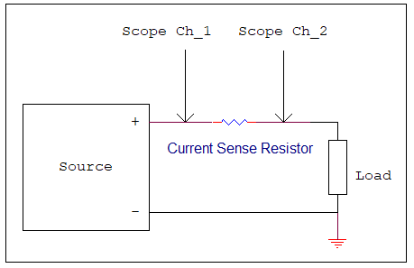
Figure 10 – High-side current measurement setup using two scope channels and math functions.
Infinite persistence
Imagine a scenario where there are some random, occasional glitches that you suspect are causing a malfunction. Without a stroke of luck, or the patience to constantly watch the scope display, there is no way to actually determine if that is really the case or not.
However, with infinite persistence mode, you can diagnose malfunctions. While in normal scope operation, a previously displayed wave form is erased each time a fresh trigger is received.
While in infinite persistence mode, this is not the case. All previous traces are kept on the screen. This makes it possible to see if a glitch has occurred over a lengthy observation period.
Know Your Instrument
All the pictures used in this article, minus the block diagrams, were captured on an actual oscilloscope. The process of capturing these pictures involved fidgeting with various settings in order to get the desired signal to properly display.
However, this was not discussed here because scopes vary in the layout of their dials, switches and other menu selections. They also vary in their math capabilities.
Even a seasoned engineer will be fumbling for a bit when trying to get a stable display on an unfamiliar scope. However, the basic steps, such as selecting the proper time base, vertical scale and trigger edge and level, are the same for all oscilloscopes. \
To learn more about oscilloscope here is a good resource.

Excellent article !