
Introduction to Audio Design for Embedded Applications
This article explores the ways to add audio capabilities to a typical small embedded system, along with the tradeoffs that are usually made in the process.

Embedded applications often need to reproduce sound. Whether you need simple prompts, chimes, rings or music clips, having the ability to reproduce pre-recorded audio can greatly enhance the UI (User Interface) of many embedded applications.
Please note that it is not the intent of this article to discuss what sounds acceptable or not, because audio “quality” is personal and subjective.
Audio Digitization Basics
Unless the sound is entirely synthesized, the original audio source is an analog signal. Remember that the real world is analog.
However, since embedded systems are digital in nature, the analog signal has to be converted to digital in order to be stored. In the end, this digitally stored and processed signal has to be played back in analog form.
Digitizing an audio signal means converting the continuous-time signal into a sequence of discrete samples. The two factors that most directly affect the storage and processing of digital audio in embedded systems are sampling rate and bit-depth, or the number of bits used to represent a single sample.
For both of these quantities, the lower they are the better it is for the use of system resources. In turn, these depend on the characteristics of the input signal.
The sampling rate is subject to the Nyquist-Shannon Sampling Theorem. It states that the minimum sampling rate (the Nyquist rate) required to reproduce a band-limited signal is twice the bandwidth of the signal. So, in order to reduce the sampling rate of the signal, simply reduce the bandwidth of the signal.
This requirement is not as not as restrictive as it appears at first glance. Even though audio signal is usually defined as having a bandwidth of 20 Hz to 20 KHz, most people are not capable of hearing a 20 KHz tone.
Certainly, if the audio output transducer, the speaker system, is not capable of reproducing such a high audio frequency, there is very little point in using a sampling rate that can accommodate this frequency.
For reference, the audio bandwidth of a regular phone is 400 to 3400 Hz. While the sound is by no means high-fidelity, users can nevertheless discern the words being spoken, and can even identify the caller’s voice. It is even possible to play fairly low-quality, but still recognizable, music over the phone.
The second factor to consider in digitizing audio signals is the bit depth. This is essentially the number of bits used to represent each sample, with the total number of possible discrete levels being 2n, where n is the number of bits.
An Analog to Digital Converter, or ADC, is typically used for this purpose. As an aside, please note that n in this case may not exactly be the number of bits stated in the specifications of the ADC.
Real ADC’s have linearization and quantization errors. Input signal conditioners such as Op-Amps can introduce even more errors.
A better estimation of the bit depth is the Effective Number Of Bits (ENOB) for the selected ADC. This number will be less than, or at most equal to, the bit width of the ADC.
Since it is generally quite difficult to accurately calculate the ENOB, a good rule of thumb is to simply assume an ENOB of 2 bits less than the published specifications of the ADC.
Using this, a 12-bit ADC is assumed to actually be a true 10-bit ADC. Of course, the greater the bit depth the less the digitalization errors. Insufficient bit depth results in an effect called quantization noise in the reproduction of the signal. This link shows what quantization errors sound like.
In embedded systems memory is organized in bytes, so the bit depth is usually a multiple of eight, such as 8-bits or 16-bits. So, even if the ADC is only capable of, say, 12-bit digitization, each sample will be stored in the next higher 8-bit memory size, which in this case is 16-bits.
It requires too much processing to store four 12-bit samples into six bytes instead of eight bytes, as in the case where each 12-bit sample is stored as sixteen bits.
Pre-Processing and Storing Audio Signals
In small embedded systems, audio is mostly stored in Linear Pulse Code Modulation, commonly known as PCM, or in WAVeform Audio (WAV) formats. These two formats are very closely related, and are the simplest of all currently available audio encoding techniques for digital processing and storage.
PCM is the technique described in the previous section. The audio signal is sampled at fixed intervals, and each sample is n bits wide, where n is the bit depth.
As an example, to store one second of music sampled at Red Book CD quality of 44.1 KHz and 16-bit bit depth, requires 705600 Bytes of data for each channel; double that for stereo. The WAV format is just PCM information with additional information such as playlist, cue points, and so on, attached. So, it is slightly larger that the raw PCM data.
If this storage requirement is not acceptable due to hardware limitations, there are several ways to reduce the size of the stored data. One is to store the audio in a compressed format such as MP3. A multitude of other formats, with lossless or lossy compression, are also available.
As mentioned before, these are not typically used in small embedded systems because the compression algorithms can be quite complex. In such cases, an external MP3 hardware decoder can be employed.
However, if the system has enough processing power and memory, for example a Raspberry Pi 4, it is quite feasible to run the MP3 decoding in the firmware.
If the source is available in analog format, then it is possible to employ analog compression techniques to reduce the dynamic range of the signal, and also to employ analog filters to reduce the bandwidth.
By reducing the dynamic range of the signal, it is possible to use a lower bit depth for each sample without introducing excessive quantization noise.
Limiting the bandwidth, on the other hand, allows for a reduction in the sampling rate. Both of these help reduce the storage requirements for a given sound clip. This is quite effective if the sound reproduction end is inherently incapable of reproducing the original signal in the first place.
For example, if the speaker is not able to produce signals higher than, say, 10 KHz, there is little point in keeping the input signal frequency components beyond this frequency.
Now, if the signal is already in digital form, then a software package such as Audacity, available here, can be used to compress and resample this signal.
This works even if the signal is originally available in analog format. In such cases, the signal can first be digitized on a desktop sound card, and then processed to reduce bandwidth and sampling rate.
Outputting Audio
Depending on the hardware, the stored audio can be output as either an analog signal, or in digital form to be further processed into actual sound.
In the first case, PCM audio can be processed through a Digital to Analog Converter, or DAC. If the storage format is already in PCM no further processing is required before sending it to the DAC.
Otherwise, in cases such as MP3 audio, it has to be converted to PCM first. The output is an analog representation of the signal. To obtain the original analog signal, the DAC output needs to be low-pass filtered to remove the sampling clock.
This is usually accomplished either with a passive or an active analog filter. One of the issues with using DACs is that if the signal is stereo, then two DACs, each with its own low-pass filter, are required.
Some microcontrollers have an I2S interface instead of built-in DACs. I2S, or Inter-IC Sound, is specifically designed to transmit audio signals, and the communication is one-way, as opposed to the somewhat similar sounding I2C communication protocol.
It uses a three-wire link to transmit stereo signals. The left and right channels are actually sequentially sent, depending on the state of the Word Select line, as shown below in figure 1. One of the interesting features of the I2S communication protocol include the fact that the SCK clock frequency is not specifically defined.
The number of bits transmitted per channel is also not specifically defined. This allows for quite a bit of flexibility in transmitting PCM audio of any sampling rate and bit depth. Incidentally, due to this flexibility, I2S has also been used to transmit other types of data besides sound.
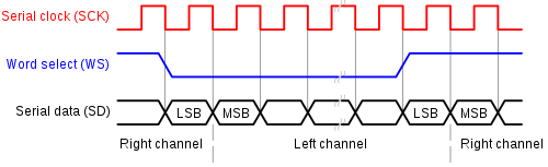
Figure 1 – I2S signaling scheme
Audio Playback
Because sound is inherently analog in nature, the transducer that reproduces the sound, essentially the speaker, is also an analog component that has to be driven with an analog signal.
Whether the analog signal is from a DAC, or a decoded I2S digital stream, it is way too weak to produce any sound of significant amplitude. So, an amplifier is needed in order to drive the transducer.
Audio amplifiers fall into two main categories: analog or digital. Analog amplifiers are further classified into class-A, or class-AB types, whereas digital audio amplifiers are generally known as class-D amplifiers.
The main advantage of a class-A is low distortion if the amplifier is well designed. Without getting into too much detail, class-A amplifiers rely on an output stage where the transistor is always biased in its linear operating point.
For a transistor, this is the state with its most linear amplification characteristics. Unfortunately, this is also the state where the transistor continuously dissipates power, whether a signal is present or not. Class-A amplifiers are usually implemented using discrete transistors, and are not typically used in embedded applications.
Class-AB amplifiers rely on an output stage that employs two transistors, or two sets of parallel-connected transistors, bipolar or MOSFET’s. One transistor conducts during the positive part of the input while the other conducts during the negative part.
During periods of no input signals, the transistors conduct minimally, thus wasting little power. Class-AB amplifiers used in embedded systems are usually in the form of a chip, and are rarely implemented using all discrete components.
The type of audio power amplifier that is most widely used in embedded applications is the Class-D type. First, the input signal is converted into a Pulse Width Modulation, or PWM, signal. In this scheme, the input signal is sampled at regular, but very short, intervals.
During each such interval, the output is fully on, or fully off, with the on to off ratio directly proportional to the amplitude of the sampled input signal at the time that particular sampling interval started. The resultant output is a stream of on/off signals of variable widths that represents the input analog signal.
When this is fed to a transistor, typically a MOSFET, its output will either be in cutoff or saturation modes, following the on/off transitions of the PWM signal. Since a transistor in either saturation or cutoff dissipates very little power, this makes the class-D amplifier very efficient.
To put this in another way, for a given power output, the size of this amplifier will be much smaller than the previous types described. That is why class-D audio power amplifiers are extensively used in embedded systems.
Note that an analog, low-pass filter is needed at the output of a class-D amplifier to remove the sampling frequency components. Since this frequency is usually quite high, the filter size can be made quite small.
There are also single chips that have both an I2S interface and a class-D power amplifier. This TI chip is one example. There are also inexpensive, ready-made modules such as this one.
For the speaker itself, the most common choice is the electrodynamic speaker.
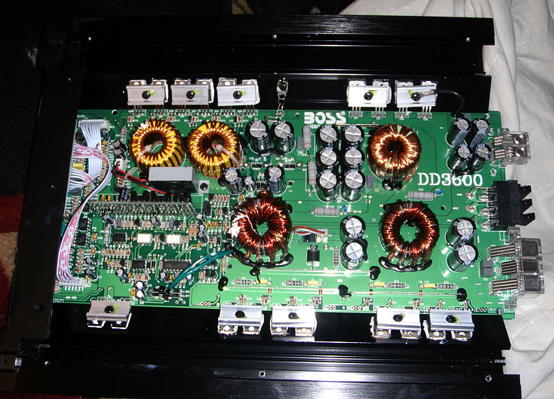
Figure 2 – Inside a Boss Audio DD3600 Class D mono block amp
The output audio signal creates a magnetic field in a coil that, in turn, interacts with a permanent magnet, causing the coil to move. The coil is actually attached to a diaphragm that displaces the air around it, creating sound. These exist in different sizes and power handling capabilities.
Also, since it is not easy to design a single speaker to handle the entire audio frequency range, high fidelity systems usually have two different speaker types to separately handle the lower-end and the higher-end of the full audio spectrum. These speakers are referred to as woofers and tweeters respectively.
There are other types of speakers as well, such as piezo speakers from TDK. Finally, for wearable products, there is a relatively new breed of very small MEMs speakers from Usound.
Conclusion
Whether you need the ability to play simple sounds, or pre-recorded music or speech, the principles outlined in this article will apply.
As shown in this article, adding music or speech capabilities to your product doesn’t necessarily require a high-performance microprocessor.
Significant audio capabilities can be easily added to embedded systems based on a variety of microcontrollers. This is especially true for systems based on microcontrollers that support the I2S digital audio serial communication standard.

Excellently explained basics of Audio. 👏👏👏
Thank you BK, I appreciate the comment.
Really great article!!
705600 bits, not bytes
Thank you for this great article (as usual).
One question: have you some suggestions to implement an equalizer in the audio output?
Thank you, Michel